Building with Mojo (Part 2): Using SIMD in Mojo

Mojo’s SIMD-first model in practice: DType, fixed-size vectors, sys.info, and vectorize.

This article is Part 2 of our ongoing series on the Mojo programming language. Part 1 introduced Mojo’s origins, design goals, and its promise to unify Pythonic ergonomics with systems-level performance.

Building with Mojo (Part 1): A Language Born for AI and Systems

Mojo is a high‑performance language. One of the main features enabling that goal is support for parallel processing at several levels:

• CPU calculations use SIMD automatically. A vectorize algorithm is available to support this data‑parallel processing at a higher level.

• Its runtime enables task‑parallel processing through automatic multithreaded code execution across multiple cores using the parallelize algorithm. This ensures maximum usage of all CPU cores.

• It supports execution on GPUs (which is intrinsically data‑parallel processing) with the same syntax used for CPU execution.

In this article we show the first way of parallelizing calculations in Mojo. Execution on GPUs will be addressed in a separate article.

We will first go deeper into what SIMD is and then demonstrate how Mojo works with it. We’ll talk about the following topics:

• What is SIMD?

• Mojo is SIMD first

• Retrieving and using SIMD system properties

• What is a SIMD vector?

• Working with SIMD vectors

• The @register_passable decorator

• Retrieving info about the host environment

• Harnessing SIMD with vectorization

The code in this article uses Python integration and calculations at compile time. We’ll discuss these topics more in depth in later articles. All code has been tested in Mojo’s latest stable version 25.4.

To follow along, first follow the instructions on https://docs.modular.com/max/get-started to install pixi. Then use pixi to create a project called simd and cd into it. We are going to let Mojo work together with Python, so we need a running Python environment inside the Mojo project. Add a recent Python version such as 3.12 to the project with the command:

$ pixi add "python==3.12"

and start a pixi shell. To add the necessary Python library, run:

$ pixi add matplotlib

What is SIMD?

SIMD is short for “Single Instruction, Multiple Data.”

This tells us that SIMD is a way to process data simultaneously (in parallel). It takes advantage of special hardware registers called SIMD or vector registers in the CPU processors of the machine. Modern CPU cores, including those in desktops, servers, and even mobile devices, contain such registers that can perform calculations simultaneously on fixed‑length vector data. This makes it possible for a single core to do up to 4, 8, 16, 32, or even 64 operations in parallel.

Their instruction sets have SIMD capabilities built in: Intel processors have SSE (Streaming SIMD Extensions) and AVX (Advanced Vector Extensions), and ARM Cortex‑A and Cortex‑R processors have the NEON SIMD instruction set.

For example, an Intel CPU with AVX‑512 has a 512‑bit vector register. This amounts to having 512/64 = 8 Float64 data items on which we can perform calculations simultaneously. The theoretical speedup is 8×, but in practice it will be lower due to memory read/write latency. The following schematic clarifies this:

Figure 1: A schematic of how SIMD works

Mojo has SIMD built in through the way its type system is set up. When you work with numerical types in Mojo, every operation is performed within SIMD registers.

Making an algorithm use SIMD fully is also called vectorizing. This is ideal for processing large amounts of data simultaneously, such as in image processing, artificial intelligence, and scientific calculations.

Mojo is SIMD first

Several languages (like C++, Rust, and so on) handle SIMD by using special libraries. But Mojo is unique in that SIMD is baked into the language: all numerical types and all built‑in mathematical functions on these types use it automatically. Python works with references (a kind of pointers) for all variables, even for simple numbers. In Mojo, numbers (and other simple values) sit on the stack and can be passed straight into SIMD registers to be processed in bulk. We don’t need to look up these values on the heap via an address as in Python.

All the numerical data types that can be used in a SIMD vector in Mojo fall under the DType umbrella. DType is a built‑in standard type defined as:

@register_passable(trivial)
struct DType

It contains the Bool type; 8‑, 16‑, 32‑, 64‑, 128‑, and 256‑bit signed and unsigned integer types (like UInt32 and Int256); and 8‑, 16‑, 32‑, and 64‑bit floating types (like BFloat16 and Float32).

For example, DType.float64 means the same as type Float64, and DType.uint32 means the same as type UInt32. Note that DType.float64 is a value, while Float64 is the real type.

Scalar[DType.float64] is another alias for the type of a single Float64 value.

The @register_passable decorator indicates that all of these types are handled through the SIMD registers.

SIMD should not be confused with parallel processing with threads executing on multiple cores. Each core has dedicated SIMD vector units, and we can take advantage of both SIMD and parallel processing to achieve massive speedup.

Retrieving and using SIMD system properties

To make the best use of the vector registers, it is important to know the SIMD capabilities of our target machine. The module sys.info contains a few functions to get that information (the results shown are for an Intel CPU with an AVX‑512 register):

from sys.info import simdbitwidth, simdbytewidth, simdwidthof

fn main():
    print(simdbitwidth())   # => 512
    print(simdbytewidth())  # => 64
    print(simdwidthof[DType.uint64]())   # => 8
    print(simdwidthof[DType.float32]())  # => 16

The function simdbitwidth shows the total number of bits that can be processed at the same time on the host system’s SIMD register. The result 512 means that we can pack 64 × 8 (= 512) bits, or 16 4‑byte numbers, or 8 8‑byte numbers together and perform a calculation on all of these with a single instruction.

The total number of bytes that can be processed at the same time is given by simdbytewidth (64 bytes on this machine).

Lastly, the function simdwidthof shows how many values of a certain type can fit into the target’s SIMD register. For example, use it to see how many UInt64s can be processed with a single instruction. On our system, the SIMD register can process 8 UInt64 or 8 Float64 or 16 Float32 values at once.

What is a SIMD vector?

SIMD is a way to process data in parallel: all items in a SIMD vector (which is basically a list of numbers) undergo the same instruction simultaneously. Simply put, instead of one instruction processing one number, one instruction processes 4, 8, 16, 32, or more numbers at a time. SIMD is used in every calculation in Mojo, so understanding it in depth is very important.

Vectors are a basic type in any systems language. Their typical syntax is like [1, 2, 3, 4], a numerical vector containing 4 elements. They are extensively used in calculations, which is why they are a first‑class type.

In Mojo, vectors are SIMD‑based and stored in stack memory, and they have a fixed size. A SIMD vector is defined as a struct with two parameters, type and size: struct SIMD[type: DType, size: Int].

Mojo allows the definition of generic structs which have parameters declared between []. Many structs from the stdlib take a type as a parameter. These parameters are processed at compile time to generate optimal code for that type.

Here is an example of a SIMD vector:

var sd = SIMD[DType.uint8, 4](1, 2, 3, 4)

Another way to define the same vector is:

var sd2: SIMD[DType.uint8, 4] = [1, 2, 3, 4]

The type of the vector’s elements is DType.uint8 or UInt8. The size or length of the vector is 4, the number of elements. Because of the hardware registers needed for SIMD, the size of a SIMD vector must be a power of 2, so 1, 2, 4, 8, and so on are all valid sizes. Vector registers are the fastest kind of memory access at the hardware level, but their number is limited, in many CPUs currently at 32. For a machine with simdbitwidth 512, the limit is 64.

To process the maximum number of values of a certain type (here Float32) simultaneously, you would use an expression like the following:

SIMD[DType.float32, simdwidthof[DType.float32]()]

This defines a SIMD vector that processes 16 Float32 values on a machine with a simdbitwidth of 512.

To explain how SIMD works, let’s compare the same operation (let’s say multiplying each element by 10) for a List with four elements 1, 2, 3, and 4, defined in Mojo as:

var lst = List[UInt8](1, 2, 3, 4)

and the SIMD vector sd from above with the same elements.

Using an ordinary List, we could use a for loop to do the multiplication, iterating over each item. Using a SIMD vector does the same work in only one operation, for all items at the same time. The following illustrates that principle:

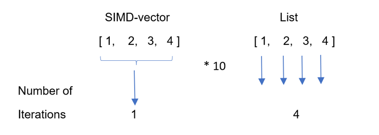
Figure 2: SIMD processing: A SIMD vector is processed in one stroke, whereas a List has to be processed item by item.

A single instruction is processed across all its items at the same time (in parallel), instead of 4 separate instructions as when we use a for loop for the list. As an analogy: visualize the array of numbers as a bus with seats. Applying SIMD, with only one instruction, we can process the entire bus in the same amount of time it would have taken to process a single number in a non‑SIMD way.

Obviously, this is faster than processing these items one by one from start to end of the list: the same calculation done with a SIMD vector is 750× faster than a corresponding NumPy array calculation.

The following code shows the difference in processing all elements for a List compared to all elements of a SIMD vector:

Processing all elements in a List and in a SIMD vector

var lst = List[UInt8](1, 2, 3, 4)  # Defining a List with 4 elements
print("[", end="")  # This print stays on the same line

# All elements of the List are processed one by one, in sequence, in a for-loop.
for ref i in lst:                  # i is a reference
    i *= 10
    print(i, end=", ")
print("]")
# => [10, 20, 30, 40, ]

var sd = SIMD[DType.uint8, 4](1, 2, 3, 4)    # Defining a SIMD vector with 4 elements
# Another way to define the same vector:
var sd2: SIMD[DType.uint8, 4] = [1, 2, 3, 4]
print(sd2)  # => [1, 2, 3, 4]

# All elements of the SIMD vector are processed simultaneously, in parallel
sd *= 10
print(sd)  # => [10, 20, 30, 40]

To multiply every element in the List lst by a factor of 10, we have to go over the list with a for loop. The index i in the for loop is a reference and is made mutable by ref; it contains the address of the corresponding List element. Nothing of the sort is needed for the SIMD vector: we can simply use its name in every operation we want to apply on it, and the processing happens over all elements at once without going through a loop.

Working with SIMD vectors

Here are some basic operations with a SIMD vector:

print(sd)  # => [1, 2, 3, 4]
print(len(sd))  # => 4
assert_equal(sd[2], 3)
sd[2] = 5
print(sd)  # => [1, 2, 5, 4]

All operators like *, /, %, ** can be applied to SIMD vectors of the same size and type; for example, multiplying two SIMD vectors of size 4 is done in one operation. Math operations on SIMD values are applied elementwise, on each individual element in the vector, but simultaneously. You can cast SIMD values to the Bool type with Bool() and then apply &, |, ^, or other boolean operators.

If you leave the () empty in the definition of a SIMD vector, you make a vector of zeros. If you fill in only one value, it is taken as the default for all elements:

var zeros = SIMD[DType.uint8, 4]()
print(zeros)  # => [0, 0, 0, 0]

var ones = SIMD[DType.uint8, 4](1)
print(ones)   # => [1, 1, 1, 1]

The math.iota function is used to fill up a SIMD vector with subsequent integers:

var numbers = SIMD[DType.uint8, 8]()
print(numbers)  # => [0, 0, 0, 0, 0, 0, 0, 0]
# Fill them with numbers from 0 to 7
numbers = math.iota[DType.uint8, 8](0)
print(numbers)  # => [0, 1, 2, 3, 4, 5, 6, 7]

numbers *= numbers
print(numbers)  # => [0, 1, 4, 9, 16, 25, 36, 49]

all is a neat function to test a condition, which can be applied to all elements at the same time:

x = SIMD[DType.uint8, 4](2, 4, 6, 8)
if all(x < 3):
    print("all elements less than 3")
else:
    print("at least one element >= 3")
# => at least one element >= 3

Some other commonly used methods are join, interleave, and shuffle:

alias dtype = DType.float32

fn main():
    var a = SIMD[dtype, 4](0.5)
    var b = SIMD[dtype, 4](2.5)

    print(a.join(b))
    # => [0.5, 0.5, 0.5, 0.5, 2.5, 2.5, 2.5, 2.5]

    print(a.interleave(b))
    # => [0.5, 2.5, 0.5, 2.5, 0.5, 2.5, 0.5, 2.5]

    var c = SIMD[DType.int8, 4](42, 108, 7, 13)
    print(c.shuffle[1, 3, 2, 0]())  # => [108, 13, 7, 42]

The join function concatenates two SIMD vectors, and interleave weaves their elements together. shuffle rearranges the elements according to the mask indices given inside the [].

The Scalar type we talked about before, defining one number, is in fact a SIMD vector of size 1:

alias Scalar = SIMD[size=1]

This is shown here:

s1 = Scalar[DType.int32](42)
s2 = SIMD[DType.int32, 1](42)
assert_equal(s1, s2)

If we combine this with what we know from the Scalar type, we can state that Int32, Scalar[DType.int32], and SIMD[DType.int32, 1] all mean the same thing. This shows again that all numerical types are intrinsically SIMD defined.

A Mojo idiom is to use the SIMD type and size as compile‑time constants. We can define the type to be used (element_type) and the number of values (group_size) as aliases, as in the following listing:

Using the SIMD type and size as compile‑time constants

from sys.info import simdwidthof
import math

# Defining type and size as aliases
alias element_type = DType.int32
alias group_size = simdwidthof[element_type]()

fn main():
    # Initialize SIMD vector numbers with aliases
    var numbers: SIMD[element_type, group_size]
    numbers = math.iota[element_type, group_size](0)
    print(numbers)  # => [0, 1, 2, 3, 4, 5, 6, 7]

Working in this way, the vectors you define fit maximally in the SIMD register, which benefits performance.

The stdlib module complex also defines a type ComplexSIMD and methods to work with complex numbers having SIMD backing.

The @register_passable decorator

Any Mojo type whose value is of type AnyTrivialRegType is register‑passable. This means that its values can be used in SIMD registers, so we know such a type can be handled faster. These are also called trivial types, like Int, Bool, and any SIMD type. By default, they are stored on the stack.

We also have a way to indicate whether a value other than DType values—for example, the fields of a struct—can be processed in SIMD registers. This is done by annotating the struct with a register_passable decorator:

@register_passable
struct Coord:
    # all fields can be passed into SIMD registers
    var x: UInt32
    var y: UInt32
    var z: UInt32

When all the individual fields of a struct can be processed in SIMD registers, the struct as a whole can be passed into registers.

The generated code for the struct will then be optimized to work more efficiently.

Because the struct in our example has only fields of trivial types, we can make this clear by using: @register_passable("trivial").

If used in combination with @fieldwise_init (which generates a constructor called __init__ for all fields), the order of the decorators is important:

@fieldwise_init
@register_passable
struct Coord:
    # …

Retrieving info about the host environment

The more you know about the host machine your program will run on, the better you can tailor your code to gain speed or save memory. For example, you may want to know the type of your CPU and which specific features it has, which OS you’re running, and so on.

Based on this info, we could execute different code when we are on macOS compared to when we are running on Linux. Mojo has this info ready for you, stored as Bool values in sys.info, as you can see in the following code (results are for a machine that runs WSL2 in Windows 11):

from sys.info import (
    os_is_linux, os_is_macos, os_is_windows,
    has_avx, has_avx2, has_avx512f, has_intel_amx,
    has_neon, has_vnni, is_apple_m1, is_apple_m2, is_apple_m3,
    _current_arch, _triple_attr,
    num_logical_cores, num_physical_cores,
    has_nvidia_gpu_accelerator,
    has_sse4
)

from sys import CompilationTarget

fn main():
    var os: String
    if os_is_linux():
        os = "linux"
    elif os_is_macos():
        os = "macOS"
    else:
        os = "windows"

    var cpu = String(_current_arch())
    var arch = String(_triple_attr())

    print("The host OS is  : ", os)
    print("Its CPU is      : ", cpu)
    print("Its Architecture: ", arch)
    print("Number of Physical Cores: ", num_physical_cores())
    print("Number of Logical Cores: ", num_logical_cores())
    # =>
    # The host OS is  :  linux
    # Its CPU is      :  alderlake
    # Its Architecture:  x86_64-unknown-linux-gnu
    # Number of Physical Cores:  12
    # Number of Logical Cores:   24

    print("CPU-features:")
    if has_sse4(): print("sse4", end=" / ")
    if has_avx():  print("avx", end=" / ")
    if has_avx2(): print("avx2", end=" / ")
    if has_avx512f(): print("avx512f", end=" / ")
    if has_intel_amx(): print("intel_amx", end=" / ")
    if has_neon(): print("neon", end=" / ")
    if is_apple_m1(): print("apple_m1")
    if has_vnni(): print("avx512_vnni", end=" / ")
    if has_nvidia_gpu_accelerator(): print("NVIDIA-GPU")

    # =>
    # CPU-features:
    # sse4 / avx / avx2 / avx512_vnni / NVIDIA-GPU

A number of functions starting with has_ or is_ give info about the processor type and capabilities of the host system, among them are:

• has_sse4(): SSE4 is the older SIMD instruction extension for x86 processors (introduced in 2006).

• has_avx(): AVX (Advanced Vector Extensions) are instructions for x86 SIMD support. They are commonly used in Intel and AMD chips (from 2011 onwards).

• has_avx2(): AVX2 (Advanced Vector Extensions 2) are instructions for x86 SIMD support, expanding integer commands to 256 bits (from 2013 onwards).

• has_avx512f(): AVX‑512 (Advanced Vector Extensions 512) added 512‑bit support for x86 SIMD instructions (from 2016 onwards).

• has_intel_amx(): AMX is an extension to x86 with instructions for special units designed for ML workloads such as TMUL, which is a matrix multiply on BF16 (from 2023 onwards).

• has_neon(): Neon (also known as Advanced SIMD) is an ARM extension for specialized instructions.

• has_vnni(): the host system has avx512_vnni.

• is_apple_m1(): The Apple M1 chip contains an ARM CPU that supports Neon 128‑bit instructions and is GPU‑accessible through the Metal API.

Newer functions are regularly added; see https://docs.modular.com/mojo/stdlib/sys/info/.

Harnessing SIMD with vectorization

At the start of the article, we defined vectorizing as making an algorithm use SIMD fully. Fortunately for us, we don’t need to worry about the “making” part: Modular (the company that creates Mojo) provides a built‑in vectorize function in the algorithm package.

In the following example we calculate 256 values of the cosine function and then plot the graph using Python matplotlib. The calculations are done in a SIMD array tmp. For storage we use an UnsafePointer called array with its load and store methods. The names defined with alias become compile‑time constants. @parameter is a decorator for the cosine closure function, which ensures that the function runs at compile time and allows cosine to capture the array pointer.

The following code is executed on a machine where simdbitwidth() is 256, so simd_with gives 4, meaning 4 Float64 values fit into the SIMD register at a time:

Vectorizing the calculation of a cosine

from math import cos, iota, pi                 # Importing the necessary functions
from memory import UnsafePointer
from algorithm import vectorize
from python import Python, PythonObject
from sys.info import simdwidthof

alias size = 256
alias element_type = DType.float64
alias simd_with = simdwidthof[element_type]()

fn main() raises:
    # 1- Calculate the cosine array using vectorization:
    # Allocate array of size elements of type element_type
    var array = UnsafePointer[element_type].alloc(size)

    @parameter   # @parameter runs the function cosine at compile time
    fn cosine[simd_width: Int](n: Int):
        # Create a simd vector tmp of size simd_width
        var tmp = iota[element_type, simd_width](n)
        # print(tmp)
        # => [0.0, 1.0, 2.0, 3.0], [4.0, 5.0, 6.0, 7.0], until [252.0, 253.0, 254.0, 255.0]
        tmp *= pi * 2 / 256.0     # Convert radians to degrees
        tmp = cos(tmp)            # Calculate cosine
        # print(tmp, end="- \n")
        # => [1.0, 0.9996991239756597, 0.9987966769554031, 0.9972932019885731],
        # [0.9951896037943114, 0.992487148217141, 0.9891874614652418, 0.9852925291318769]
        # until [0.9948724987092192, 0.9970539358757885, 0.9986353937937995, 0.9996159208177102]
        array.store(n, tmp)       # Store the 4 calculated values in the UnsafePointer

    vectorize[cosine, simd_width](size)   # Vectorize the calculation

    # 2- Plot the cosine array using Python
    try:
        var plt = Python.import_module("matplotlib.pyplot")
        var graph = Python.list()
        for i in range(size):
            graph.append(array.load(i))
        plt.plot(graph)
        plt.show()
    except:
        print("error in plotting")

vectorize is called as:

vectorize[cosine, simd_width](size)

which here is:

vectorize[cosine, 4](256)

vectorize creates a loop calling cosine 64 times, 4 values at a time.

The cosine function is defined as:

fn cosine[simd_width: Int](n: Int)

and will be called with these values:

cosine[4](256)

Apart from the normal arguments enclosed within round brackets (), both of these functions also have data enclosed within square brackets []. These are called parameters. If needed, these are calculated at compile time and then stored as constants to use during runtime execution.

The net effect of vectorizing is that, on a machine with a SIMD register size of 256, this will set 4 Float64 values on each iteration, as we can see when we display tmp. This optimizes the effectiveness of the SIMD operations. The tmp values go from n to (n + simd_width – 1), where n varies from 0 to 64.

This is the resulting plot:

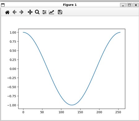
Figure 3: (Plot showing the cosine function)

The example from the previous section shows that vectorization simplifies SIMD‑optimized loops. Here is the definition of vectorize from the stdlib:

vectorize[origins: origin.set, //, func: fn[Int](Int) capturing -> None, simd_width: Int, /, *, unroll_factor: Int = 1](size: Int)

Notice that vectorize is a higher‑order function, which contains as a parameter a function with signature func: fn[Int](Int) capturing -> None. It has one Int parameter and an Int argument. Our cosine function conforms to that signature, with simd_with as parameter and n as argument.

Vectorization works by mapping a function across a range from 0 to size, incrementing by simd_width at each step. The remainder of size % simd_width, if not 0, will then run in separate iterations.

Up next:

Building with Mojo (Part 3): Python and Mojo

---

© 2025 Ivo Balbaert. All rights reserved.